Toy example II: Adding solar production, and a limit on the grid connection

So far we haven’t taken into account any other devices that consume or produce electricity. The battery was free to use all available capacity (which was 500 kVA, both its own maximum charge/discharge rate, and the maximum grid capacity).

What if other devices will be using some of that capacity? Our schedules need to reflect that, so we stay within given limits.

We will now add solar production forecast data and then ask for a new schedule, to see the effect of solar production on the available headroom for the battery (when it plans to discharge). When solar production is high, less battery output can be send to the grid, as the total site power (battery + solar) cannot exceed the site-power-capacity.

How does it work?

• We will tell FlexMeasures to take the solar production into account (using the inflexible-device-sensors flex-context field).

• The battery’s power capacity is not the limiting factor, but the site-power-capacity of the building (already a flex-context field, see Toy example I: Scheduling a battery, from scratch).

• The flows of the building’s child assets are summed up on building level, and that constraint now will play a role.

Adding PV production forecasts

First, we’ll create a new CSV file with solar forecasts (MW, see the setup for sensor 3 in part I of this tutorial) for tomorrow.

$ TOMORROW=$(date --date="next day" '+%Y-%m-%d')
$ echo "Hour,Price
$ ${TOMORROW}T00:00:00,0.0
$ ${TOMORROW}T01:00:00,0.0
$ ${TOMORROW}T02:00:00,0.0
$ ${TOMORROW}T03:00:00,0.0
$ ${TOMORROW}T04:00:00,0.01
$ ${TOMORROW}T05:00:00,0.03
$ ${TOMORROW}T06:00:00,0.06
$ ${TOMORROW}T07:00:00,0.1
$ ${TOMORROW}T08:00:00,0.14
$ ${TOMORROW}T09:00:00,0.17
$ ${TOMORROW}T10:00:00,0.19
$ ${TOMORROW}T11:00:00,0.21
$ ${TOMORROW}T12:00:00,0.22
$ ${TOMORROW}T13:00:00,0.21
$ ${TOMORROW}T14:00:00,0.19
$ ${TOMORROW}T15:00:00,0.17
$ ${TOMORROW}T16:00:00,0.14
$ ${TOMORROW}T17:00:00,0.1
$ ${TOMORROW}T18:00:00,0.06
$ ${TOMORROW}T19:00:00,0.03
$ ${TOMORROW}T20:00:00,0.01
$ ${TOMORROW}T21:00:00,0.0
$ ${TOMORROW}T22:00:00,0.0
$ ${TOMORROW}T23:00:00,0.0" > solar-tomorrow.csv

Then, we read in the created CSV file as beliefs data. This time, different to above, we want to use a new data source (not the user) ― it represents whoever is making these solar production forecasts. We create that data source first, so we can tell flexmeasures add beliefs to use it. Setting the data source type to “forecaster” helps FlexMeasures to visually distinguish its data from e.g. schedules and measurements.

Note

The flexmeasures add source command also allows to set a model and version, so sources can be distinguished in more detail. But that is not the point of this tutorial. See flexmeasures add source --help.

$ flexmeasures add source --name "toy-forecaster" --type forecaster
Added source <Data source 4 (toy-forecaster)>
$ flexmeasures add beliefs --sensor 3 --source 4 solar-tomorrow.csv --timezone Europe/Amsterdam
Successfully created beliefs

The one-hour CSV data is automatically resampled to the 15-minute resolution of the sensor that is recording solar production. We can see solar production in the FlexMeasures UI:

Note

The flexmeasures add beliefs command has many options to make sure the read-in data is correctly interpreted (unit, timezone, delimiter, etc). But that is not the point of this tutorial. See flexmeasures add beliefs --help.

Trigger an updated schedule

Now, we’ll reschedule the battery while taking into account the solar production (forecast) as an inflexible device. This will have an effect on the available headroom for the battery, given the site-power-capacity limit discussed earlier.

CLIAPIFlexMeasures Client

$ flexmeasures add schedule \
    --sensor 2 \
    --start ${TOMORROW}T07:00+01:00 \
    --duration PT12H \
    --soc-at-start 50% \
    --flex-context '{"inflexible-device-sensors": [3]}'
    --flex-model '{"soc-min": "50 kWh"}' \
New schedule is stored.

We can see the updated scheduling in the FlexMeasures UI:

The graphs page for the battery now shows the solar data, too:

Though this schedule is quite similar, we can see that it has changed from the one we computed earlier (when we did not take solar into account).

First, during the sunny hours of the day, when solar power is being send to the grid, the battery’s output (at around 9am and 11am) is now lower, as the battery shares the site-power-capacity with the solar production. In the evening (around 7pm), when solar power is basically not present anymore, battery discharging to the grid is still at its previous levels.

Second, charging of the battery is also changed a bit (around 10am), as less can be discharged later.

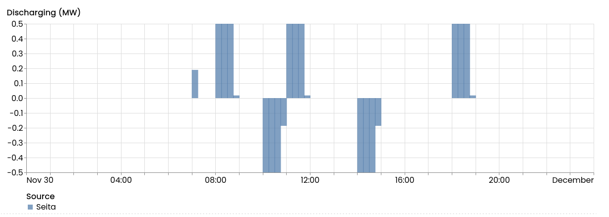
Moreover, we can use reporters to compute the capacity headroom (see Toy example V: Computing reports for more details). The image below shows that the scheduler is respecting the capacity limits.

In the case of the scheduler that we ran in the previous tutorial, which did not yet consider the PV, the discharge power would have exceeded the headroom:

Note

You can add arbitrary sensors to a chart using the asset UI or the attribute sensors_to_show. See Assets for more.

A nice feature is that you can check the data connectivity status of your building asset. Now that we have made the schedule, both lamps are green. You can also view it in FlexMeasures UI:

We hope this part of the tutorial shows how to incorporate a limited grid connection as well as other energy data streams rather easily with FlexMeasures.

This tutorial showed a quick way to add an inflexible load (like solar power) and a grid connection. In A flex-modeling tutorial for storage: Vehicle-to-grid, we will temporarily pause giving you tutorials you can follow step-by-step. We feel it is time to pay more attention to the power of the flex-model, and illustrate its effects.